Bayesian Linear Travel-Time Tomography
Seismic tomography uses measured arrival times to build a picture of the subsurface. Many different models can fit the same data, so it matters how uncertain the resulting image is, and a lot of that uncertainty is set by where the sources and receivers are placed. This project looks at both questions in a deliberately simple setting where everything can be computed exactly. The slowness field is discretised on a uniform grid, travel times are modelled as straight-ray line integrals, and the prior and noise are Gaussian, so the posterior has a closed form and no sampling or approximation error gets mixed in with the results.
There are two main experiments, preceded by a baseline reconstruction and a calibration check. The baseline builds the forward model and runs a single reconstruction of a fixed slowness field as a sanity check. The calibration check repeatedly draws the true field from the prior, ensuring the model is correctly specified by construction, and verifies that the posterior is exactly calibrated. Experiment I, like the baseline, holds the true field fixed, as it would be in a real survey, and compares the posterior uncertainty with the scatter from repeated noise. Experiment II keeps the field, prior and noise level fixed and compares different sensor configurations.
All project code can be found here.
1. The forward model Link to heading
We work on a square cross-section of the subsurface, $\Omega = [0, W] \times [0, W]$. Sources sit along the left edge and receivers along the right edge, the standard crosshole geometry of two vertical boreholes, and every source is joined to every receiver by a ray (Figure 1).
The medium is described by its slowness $s(\mathbf{x}) = \frac{1}{v(\mathbf{x})}$, the reciprocal of the local wave speed. In the high-frequency regime the first-arrival time $T(\mathbf{x})$ from a source satisfies the eikonal equation
Rays are the curves everywhere tangent to $\nabla T$. Along a ray with unit tangent $\hat{\mathbf{t}} = \frac{\nabla T}{\lvert \nabla T \rvert}$ and arc length $\ell$, the chain rule gives $\frac{\mathrm{d}T}{\mathrm{d}\ell} = \nabla T \cdot \hat{\mathbf{t}} = \lvert \nabla T \rvert = s$. Integrating along the ray $L_i$ from source to receiver gives the travel time
The eikonal equation contains no material property other than $s$: once the slowness field is known, both the arrival times and the ray paths are determined, so $s$ is the only thing we need to know about the medium to describe how a wave travels through it. Writing the problem in slowness rather than velocity is also what makes travel time an integral of the unknown itself. Nor does $s$ depend on the energy the wave carries. For small strains in a linear elastic medium, wave speed is fixed by the elastic moduli and density of the rock (for P-waves, $v_p = \sqrt{\frac{K + \frac{4}{3}\mu}{\rho}}$), and the speed of a wavefront of a linear equation does not depend on the amplitude of the solution. This fails close to a large source or at very high strain, but not for the small-strain waves recorded at receivers in a tomography survey.
The ray paths themselves depend on $s$, since rays bend towards faster rock, and this makes the map from $s$ to travel times nonlinear. We therefore make the straight-ray approximation: each $L_i$ is fixed in advance as the straight segment between its source and receiver. This keeps the forward model linear, and is reasonable when velocity contrasts are mild.
We partition $\Omega$ into a uniform $n \times n$ grid of square cells and take $s$ to be constant, $s_j$, in cell $j$. For $m$ rays, the line integral then becomes the linear system
where
The sensitivity matrix $A$ depends only on the geometry and is computed once, exactly, by grid traversal (Figure 2). Because cells are square, any directional structure in the results comes from the acquisition geometry and the prior, not from the grid.
Summing each column of $A$ gives the total ray length through each cell (Figure 3).
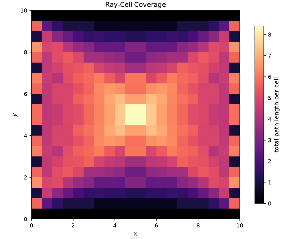
Coverage is uneven, and in every configuration studied here there are fewer rays than cells, so $A$ is rank-deficient: some slowness patterns leave the travel times unchanged. The data alone cannot determine $\mathbf{s}$.
2. Observation model and prior Link to heading
The measured travel times are the exact travel times through the true field, corrupted by independent Gaussian picking errors:
The prior supplies the information the data cannot, in particular in the null space of $A$:
where $\mathbf s_0 = s_{\mathrm{bg}} \mathbf{1}$ is a homogeneous background and $C_s$ is the squared-exponential covariance with entries
with $\mathbf x_j$ the centre of cell $j$. This covariance encodes smoothness on the length scale $\ell$. The jitter $\epsilon$ is needed because the squared-exponential matrix is positive definite in exact arithmetic but numerically near-singular on a fine grid, and its Cholesky factorisation fails without it.
3. The posterior Link to heading
With a linear forward map and Gaussian prior and noise, the posterior is exactly Gaussian,
where
This is the same linear-Gaussian update as a Kalman filter or Gaussian-process regression. Equivalently,
where the gain is
No matrix is inverted explicitly: the precision $C_{\mathrm{post}}^{-1}$ is factorised once by Cholesky, and the posterior mean follows from triangular solves.
4. Parameters Link to heading
The following values are used throughout. Acquisition layouts differ between sections and are given with each one.
| Parameter | Symbol | Value |
|---|---|---|
| Domain side length | $W$ | 10 |
| Grid resolution (cells per side) | $n$ | 20 |
| Background slowness | $s_{\mathrm{bg}}$ | 1.0 |
| Prior marginal variance | $\tau^2$ | 0.04 |
| Prior correlation length | $\ell$ | 2.0 |
| Covariance jitter | $\epsilon$ | $10^{-6}\tau^2$ |
| Noise standard deviation | $\sigma$ | 0.02 |
The baseline reconstruction and Experiments I and II use a fixed true field consisting of two Gaussian anomalies on the background,
where the anomaly width and centres are
and the field is evaluated at the cell centres. The centres are placed at $0.475W$ rather than $\frac{W}{2}$ because, for $n = 20$, the line $y = \frac{W}{2}$ is a cell boundary.
5. Baseline reconstruction Link to heading
The baseline runs the full chain once: build $A$, generate the fixed truth, add one draw of noise, and compute the posterior.
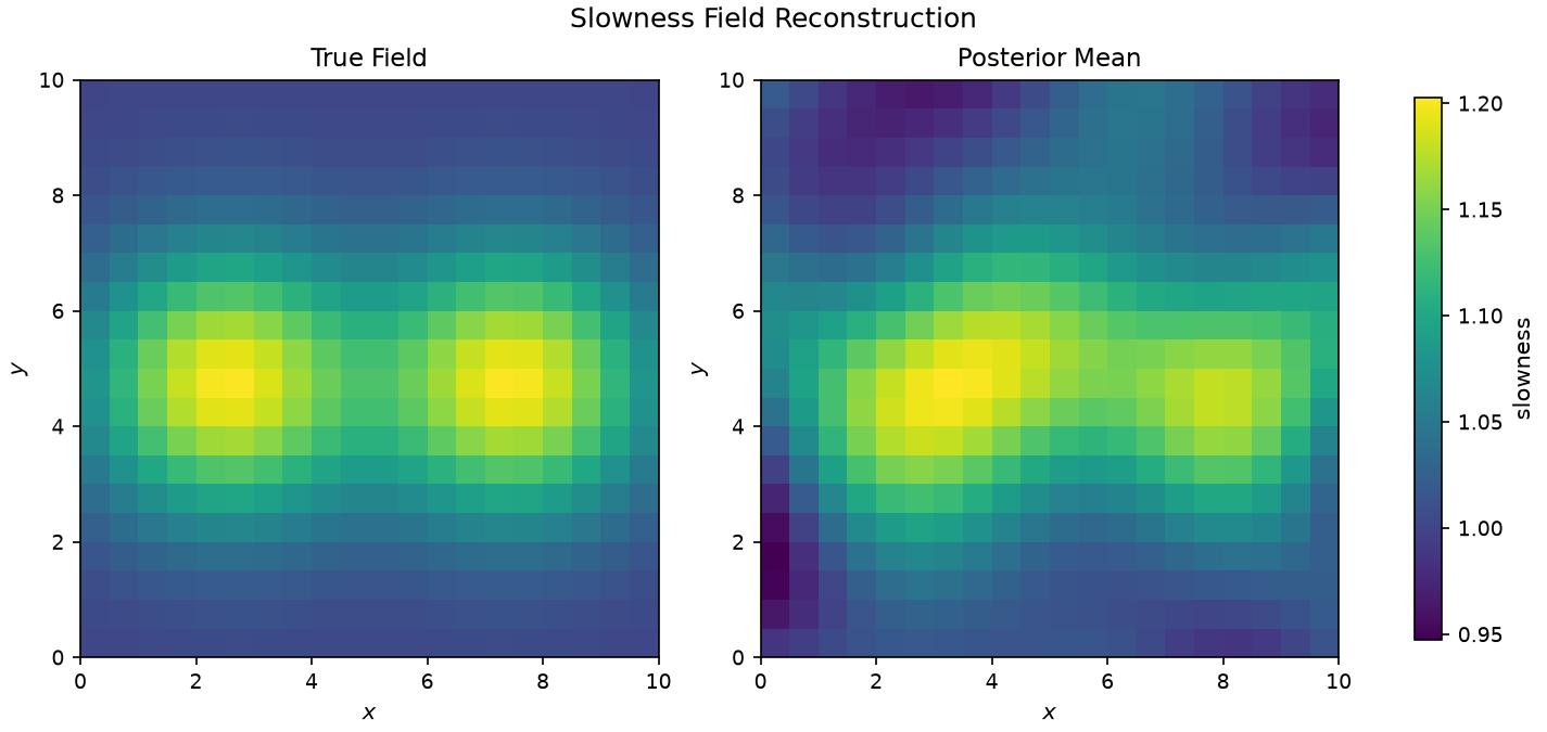
Both anomalies are recovered in the right places, but they are smeared horizontally towards each other, with small artefacts against the left and right edges. This is what the geometry predicts. Every crosshole ray crosses the domain from side to side at a moderate angle, and a travel time cannot tell where along its path a delay was picked up, so horizontal structure is poorly constrained.
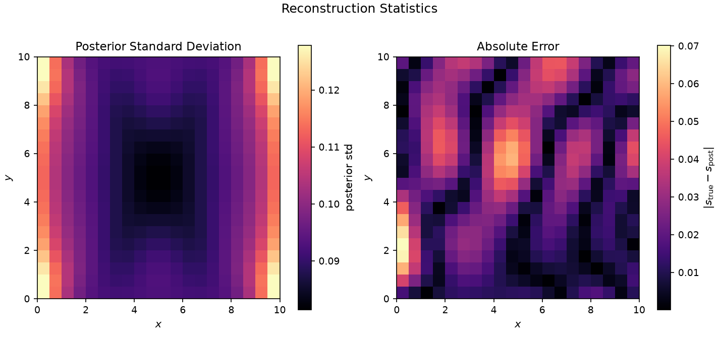
The posterior standard deviation mirrors the ray coverage of Figure 3: smallest at the centre and largest in the columns beside the boreholes. The unsampled top and bottom strips are not the most uncertain cells, because the prior correlation length spans several cells. Since $C_{\mathrm{post}}$ depends only on $A$, $C_s$ and $\sigma$, this map is a property of the survey design, available before any data exist.
6. Calibration check: the correctly specified model Link to heading
Here the true field is drawn from the prior itself, $\mathbf s_{\mathrm{true}} \sim \mathcal{N}(\mathbf s_0, C_s)$, and the data from the assumed likelihood. Generative and inference models then agree by construction, so the global Mahalanobis error
must follow $\chi^2_{n^2} = \chi^2_{400}$, and the marginal credible intervals $s_{\mathrm{post},j} \pm z_{1-\frac{\alpha}{2}} \sigma_{\mathrm{post},j}$, with $\sigma_{\mathrm{post},j}^2$ the $j$-th diagonal entry of $C_{\mathrm{post}}$, must contain the truth at their nominal rate $1 - \alpha$. This cannot fail unless the implementation is wrong, so it tests the software in the spirit of simulation-based calibration (Talts et al., 2018). Appendix A sets out why the two senses of “calibrated” in this report must be kept apart.
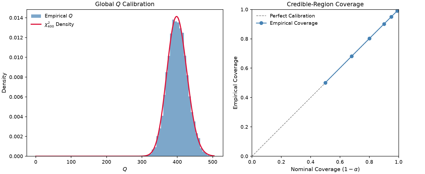
Over 1000 independent realisations, $Q$ follows $\chi^2_{400}$ and the intervals cover at their nominal rates.
7. Experiment I: a fixed truth Link to heading
A real subsurface is one particular field, not a draw from a prior. Experiment I therefore holds the truth fixed and resamples only the noise, over 1000 realisations, with $N_s = N_r = 12$ sources and receivers ($m = 144$ rays). Nothing now guarantees $Q \sim \chi^2_{400}$.
For a fixed truth the error splits into a deterministic regularisation bias and a noise-driven part,
where
is the same in every realisation. Only $K\boldsymbol{\varepsilon}$ varies, with covariance
The repeated-noise covariance $V_{\mathrm{post}}$ is not $C_{\mathrm{post}}$: the posterior covariance also carries the prior’s uncertainty about which field is true, and with the truth fixed that component is absent. Taking the expectation of $Q$ over the noise gives
The first term is the trace of the model resolution matrix $R = KA$, the effective number of parameters the data resolve. Its eigenvalues lie in $[0, 1)$ and at most $\operatorname{rank}(A) \le m$ are nonzero, so with 144 rays it cannot approach 400. The second term depends on the truth. Averaged over truths drawn from the prior it supplies exactly the remaining $400 - \operatorname{tr}(KA)$, recovering the calibration check of Section 6 (Appendix B).
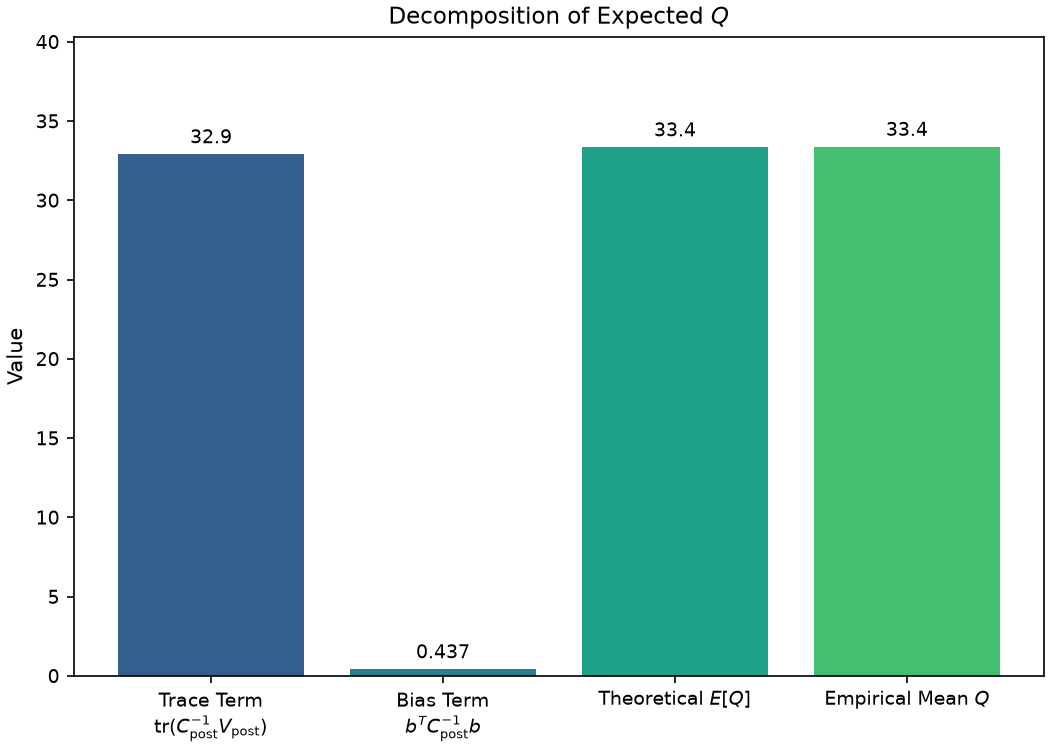
The prediction matches the simulation, and the error is almost entirely noise-driven: for this truth the bias term is small. Compared with the $\chi^2_{400}$ benchmark of the calibration check, $Q$ is an order of magnitude too small.
7.1 Coverage Link to heading
The marginal credible intervals cover the fixed truth more often than their nominal level, at every level tested:
| Nominal coverage | 0.99 | 0.95 | 0.90 | 0.80 | 0.68 | 0.50 |
|---|---|---|---|---|---|---|
| Empirical coverage | 1.0000 | 1.0000 | 1.0000 | 0.9996 | 0.9972 | 0.9717 |
Under repeated noise the estimate in cell $j$ scatters according to the diagonal of $V_{\mathrm{post}}$, while the interval is built from the diagonal of $C_{\mathrm{post}}$. The ratio
is the expected repeated-noise standard deviation of the standardised error in cell $j$; it averages about 0.27 across cells at this geometry and, like the trace term, does not depend on the truth. The intervals are therefore several times wider than the actual repeat-survey scatter, and with a small bias they over-cover. This conclusion is specific to this truth: for a field the prior describes poorly, the bias term can dominate and the intervals could under-cover instead.
8. Experiment II: acquisition geometry Link to heading
Experiment II holds the truth, prior and noise level fixed and changes only where the sources and receivers sit. Four per-edge layouts are built from the interior grid $u_i = \frac{i}{N+1}$, $i = 1, \dots, N$, with the same positions used for sources and receivers:
Smaller $\gamma$ pushes sensors towards the ends of the edge; $\gamma = 1$ recovers the uniform layout.
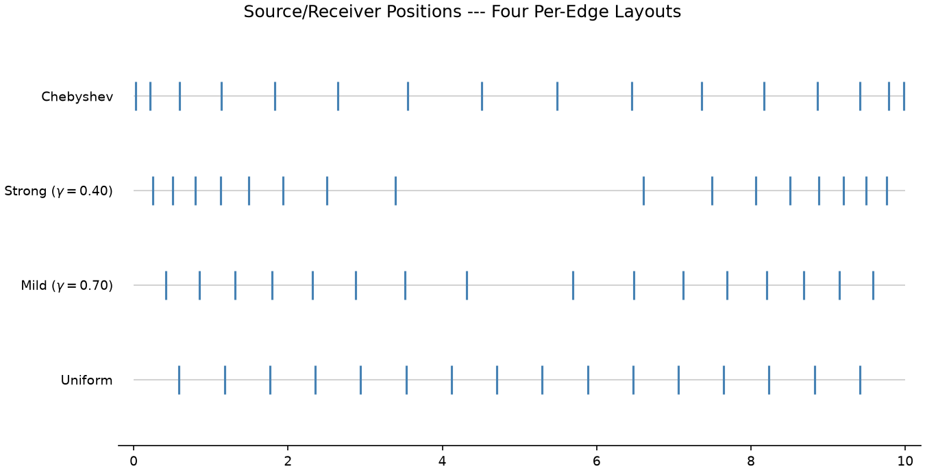
The clustered layouts open a gap in the middle of each edge that widens as $\gamma$ decreases, while the Chebyshev layout keeps sensors along the whole edge but packs them more densely towards the ends.
The two-edge designs use $N = 16$ ($m = 256$ rays). The three-edge designs add a third instrumented edge (Figure 9): $N = 12$ on each borehole, plus five nodes spaced uniformly along the top edge $y = W$, each joined to every source and every receiver, giving $m = 144 + 60 + 60 = 264$ rays.
Reconstructions are compared by the relative error
over ten independent master seeds of 200 repetitions each, with the noise paired across designs within each repetition (Appendix C).
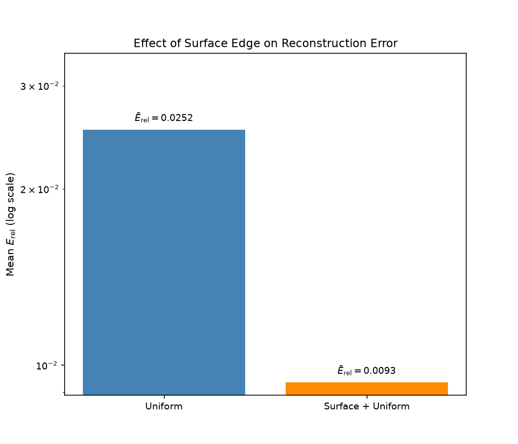
Adding the surface edge to the uniform layout cuts the mean relative error from 0.0252 to 0.0093, for essentially the same number of rays. Crosshole rays all cross the domain from side to side; the surface rays cross it steeply, and constrain exactly the horizontal structure the crosshole data could not.
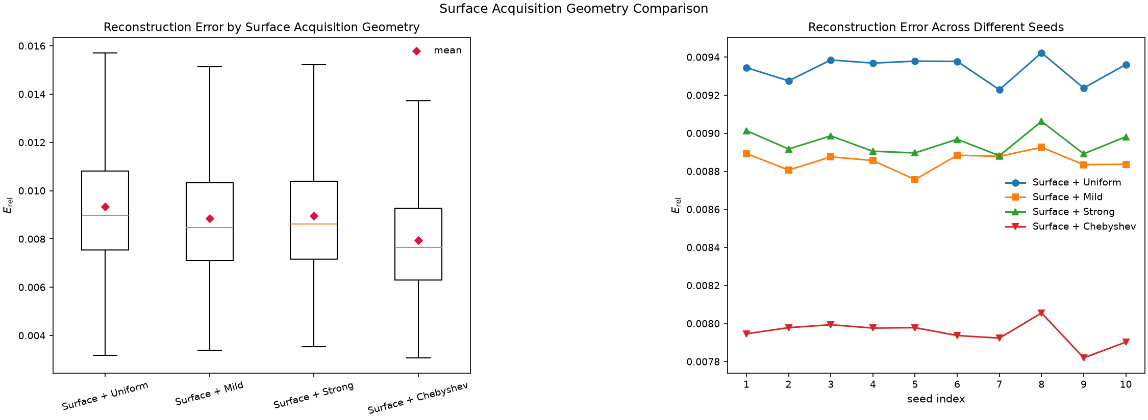
With the surface edge in place, changing the spacing along the boreholes moves the error far less than adding the edge did. The Chebyshev layout gives the lowest error at every one of the ten seeds, so the rest of this section looks at its reconstruction in more detail.
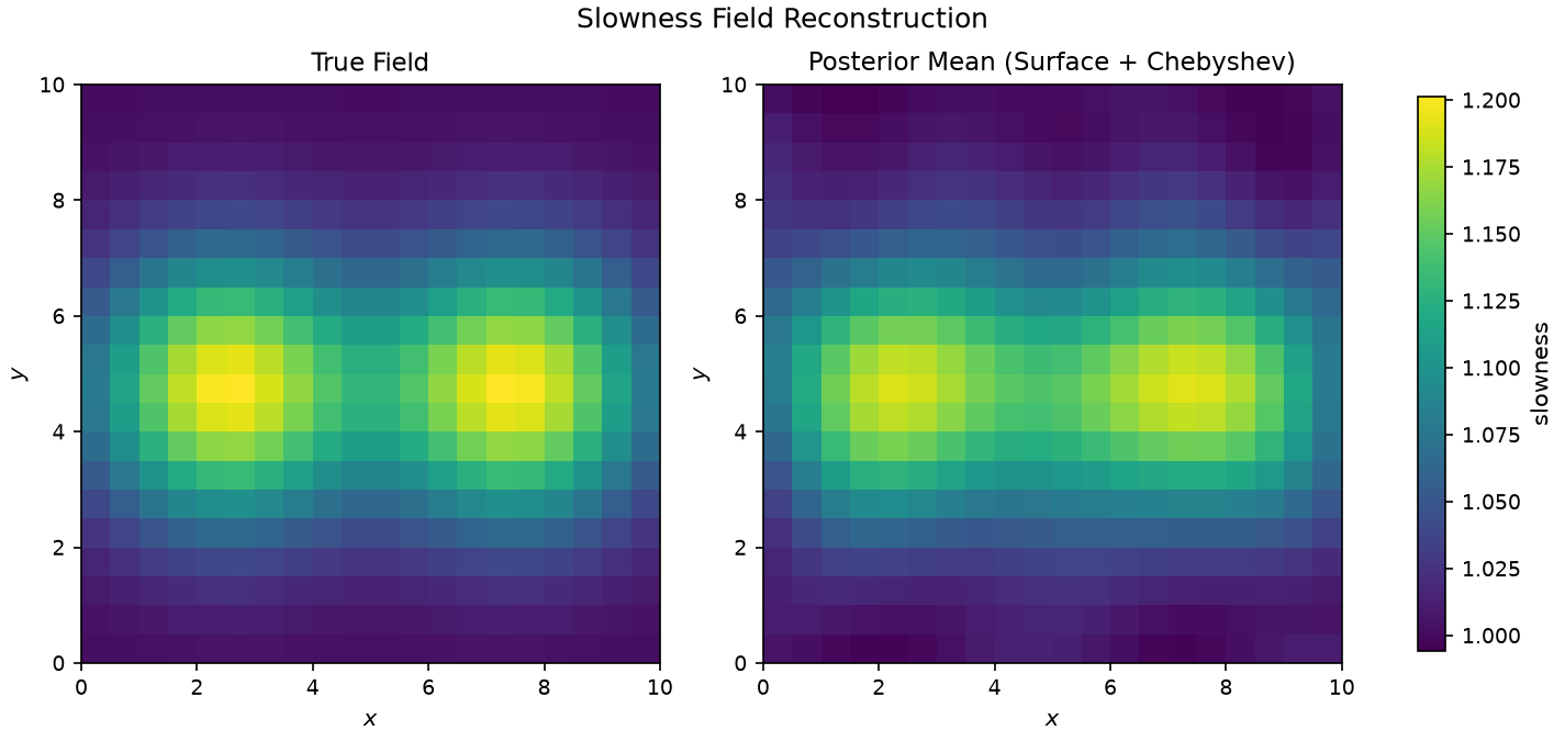
The two anomalies now come out as separate features, and most of the horizontal smearing in the baseline reconstruction (Figure 4) is gone. The steep surface rays have resolved the horizontal structure that the crosshole data left ambiguous.
The same improvement shows up in the uncertainty. Figure 13 compares the posterior standard deviation and the absolute error of the Chebyshev layout with surface edge against the uniform two-edge layout.
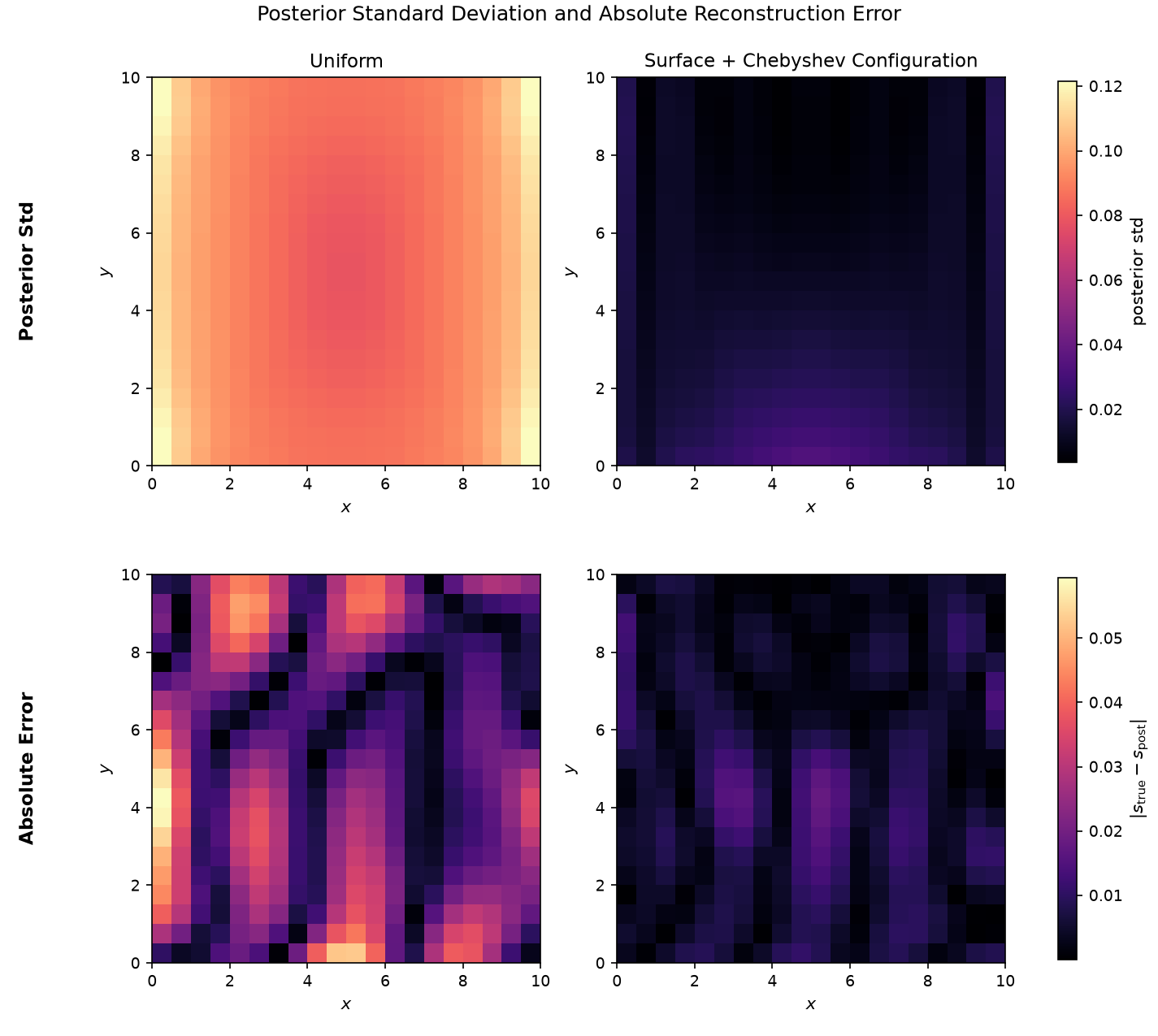
For the two-edge layout the standard deviation is high across the domain and highest beside the boreholes, the same pattern as in the baseline (Figure 5). With the surface edge it is much lower across the domain, and the remaining uncertainty is concentrated towards the bottom of the domain, the one edge that carries no instruments and is furthest from the surface array. The error maps agree: the two-edge layout has large errors along the left edge and in vertical bands, while the errors with the surface edge are small throughout.
9. Discussion Link to heading
A Bayesian posterior standard deviation is exact for the question “how uncertain is this cell, averaged over every subsurface the prior considers plausible?” It is not automatically the answer to “how much would this cell change if the same ground were surveyed again?” For the field studied here the first overstates the second, so the credible intervals are conservative; how large the gap is, and even its sign, depends on how well the prior describes the actual geology. The decomposition in Section 7 means that gap can be computed directly.
On survey design, viewing angle matters much more than sensor spacing. Rays that all travel in similar directions cannot resolve structure along those directions, however the sensors are arranged, and combining borehole instruments with a surface array is the practical way to add the missing angles.
10. Scope Link to heading
This is a controlled linear model, not a full seismic inversion. It excludes curved rays, attenuation, anisotropy, frequency-dependent effects, wave-equation simulation and non-Gaussian likelihoods, and uses a single prior and noise specification, with no controlled prior- or noise-misspecification experiment. The fixed-truth results concern one field. Experiment II compares a small set of predetermined layouts at one ray count and resolution; it does not try to find an optimal design. In return for these simplifications the posterior is exact, so any discrepancy has to come either from the implementation, which the calibration check rules out, or from the statistics, which Experiment I explains.
References Link to heading
Talts, S., Betancourt, M., Simpson, D., Vehtari, A. and Gelman, A. (2018). Validating Bayesian inference algorithms with simulation-based calibration. arXiv:1804.06788.
Appendix A. Two meanings of “calibrated” Link to heading
In the calibration check (Section 6) the truth is drawn from the prior the inversion assumes, so conditional on the data $\mathbf s_{\mathrm{true}} - \mathbf s_{\mathrm{post}} \sim \mathcal{N}(\mathbf{0}, C_{\mathrm{post}})$ exactly. The posterior is then calibrated in the sense of being right on average over the fields the prior considers plausible, and $Q \sim \chi^2_{n^2}$ is guaranteed by the model’s self-consistency. In Experiment I (Section 7) the truth is a fixed field, and whether the posterior describes repeat-survey uncertainty for that field must be checked directly; there is no general guarantee. Neither result should be stated as “the posterior is calibrated” without saying which sense is meant.
The per-cell standardised errors $z_j = \frac{s_{\mathrm{true},j} - s_{\mathrm{post},j}}{\sigma_{\mathrm{post},j}}$ from a single reconstruction are spatially correlated, through the prior and through the posterior update. Pooling them across cells and testing the pool against $\mathcal{N}(0, 1)$ treats dependent values as independent, and such a test rejects even when model and code are both correct. Each realisation instead contributes one value of $Q$, and values of $Q$ from independent realisations can be pooled legitimately; this is why calibration in this report is assessed using $Q$ and coverage.
Appendix B. Recovering the calibration check from the decomposition Link to heading
From the definition of $C_{\mathrm{post}}$, $C_{\mathrm{post}}^{-1} = \frac{1}{\sigma^2}A^\top A + C_s^{-1}$, so $I - KA = C_{\mathrm{post}} C_s^{-1}$. If $\mathbf s_{\mathrm{true}} \sim \mathcal{N}(\mathbf s_0, C_s)$, the bias $\mathbf{b} = C_{\mathrm{post}} C_s^{-1} (\mathbf s_{\mathrm{true}} - \mathbf s_0)$ has covariance $C_{\mathrm{post}} C_s^{-1} C_{\mathrm{post}}$, and
Adding the trace term gives $\mathbb{E}[Q] = n^2$, the mean of $\chi^2_{n^2}$.
Appendix C. Paired noise and master seeds Link to heading
Within each repetition of Experiment II, every design receives the same standardised noise draw, so differences between designs are not confounded by unrelated noise. A design with more rays than the shared draw takes its additional entries from an independent stream keyed to that design, so adding or removing a design never changes another design’s noise. The comparison is repeated over ten independent master seeds of 200 paired repetitions each; each point in the right panel of Figure 11 is one seed’s mean over its 200 repetitions.